6-2. Implementation of variational quantum eigensolver (VQE) using Qulacs

In this section, we show an example of running the variational quantum eigensolver (VQE) on a simulator using Qulacs for a quantum chemical Hamiltonian obtained using OpenFermion and PySCF, and searching the ground state.

requirements

• qulacs

• openfermion

• openfermion-pyscf

• pyscf

• scipy

• numpy

Install and Import of required packages

## Run if required libraries are not installed
## If you run on Google Colaboratory, igore the warning 'You must restart the runtime in order to use newly installed versions.'
## If you restart runtime, calculation may crash.
!pip install qulacs pyscf openfermion openfermionpyscf

## Run only in Google Colaboratory or (Linux or Mac) jupyter notebook environment
## Qulacs errors will be output normally.
!pip3 install wurlitzer
%load_ext wurlitzer

import qulacs
from openfermion.transforms import get_fermion_operator, jordan_wigner
from openfermion.linalg import get_sparse_operator #If you have an error, please update openfermion later than version 1.0.0
from openfermion.chem import MolecularData
from openfermionpyscf import run_pyscf
from scipy.optimize import minimize
from pyscf import fci
import numpy as np
import matplotlib.pyplot as plt

Creation of Hamiltonian

Using the same procedure as in the previous section, Hamiltonian is calculated by PySCF .

basis = "sto-3g"
multiplicity = 1
charge = 0
distance  = 0.977
geometry = [["H", [0,0,0]],["H", [0,0,distance]]]
description  = "tmp"
molecule = MolecularData(geometry, basis, multiplicity, charge, description)
molecule = run_pyscf(molecule,run_scf=1,run_fci=1)
n_qubit = molecule.n_qubits
n_electron = molecule.n_electrons
fermionic_hamiltonian = get_fermion_operator(molecule.get_molecular_hamiltonian())
jw_hamiltonian = jordan_wigner(fermionic_hamiltonian)

Convert Hamiltonian into qulacs Hamiltonian

In Qulacs, observable like Hamiltonian is treated with Observable class. There is a function to convert OpenFermion Hamiltonian into Qulacs Observable named create_observable_from_openfermion_text. Lets’s use this.

from qulacs import Observable
from qulacs.observable import create_observable_from_openfermion_text
qulacs_hamiltonian = create_observable_from_openfermion_text(str(jw_hamiltonian))

compose ansatz

Here, we compose a quantum circuit on Qulacs. The quantum circuits were modeled after those used in experiments with superconducting qubits (A. Kandala et. al. , “Hardware-efficient variational quantum eigensolver for small molecules and quantum magnets“, Nature 549, 242–246).

from qulacs import QuantumState, QuantumCircuit
from qulacs.gate import CZ, RY, RZ, merge

depth = n_qubit

def he_ansatz_circuit(n_qubit, depth, theta_list):
    """he_ansatz_circuit
    Returns hardware efficient ansatz circuit.

    Args:
        n_qubit (:class:`int`):
            the number of qubit used (equivalent to the number of fermionic modes)
        depth (:class:`int`):
            depth of the circuit.
        theta_list (:class:`numpy.ndarray`):
            rotation angles.
    Returns:
        :class:`qulacs.QuantumCircuit`
    """
    circuit = QuantumCircuit(n_qubit)
    for d in range(depth):
        for i in range(n_qubit):
            circuit.add_gate(merge(RY(i, theta_list[2*i+2*n_qubit*d]), RZ(i, theta_list[2*i+1+2*n_qubit*d])))
        for i in range(n_qubit//2):
            circuit.add_gate(CZ(2*i, 2*i+1))
        for i in range(n_qubit//2-1):
            circuit.add_gate(CZ(2*i+1, 2*i+2))
    for i in range(n_qubit):
        circuit.add_gate(merge(RY(i, theta_list[2*i+2*n_qubit*depth]), RZ(i, theta_list[2*i+1+2*n_qubit*depth])))

    return circuit

Define VQE cost function

As explained in chapter 5-1, VQE obtaions an approximate ground state by minimizing the following expectation of Hamiltonian of a state \(|\psi(\theta)\rangle = U(\theta)|0\rangle\) which is output from quantum circuit \(U(\theta)\) with a parameter .

\[\langle H (\theta)\rangle = \langle\psi(\theta)|H|\psi(\theta)\rangle\]

def cost(theta_list):
    state = QuantumState(n_qubit) #prepare |00000>
    circuit = he_ansatz_circuit(n_qubit, depth, theta_list) #create a quantum circuit
    circuit.update_quantum_state(state) #apply to a quantum circuit
    return qulacs_hamiltonian.get_expectation_value(state) #calculate the expectation of a Hamiltonian

Execute VQE

Now that we’re ready, let’s run VQE. For optimization, the BFGS method implemented in scipy is used, and the initial parameters are randomly selected. It should finish in tens of seconds.

cost_history = []
init_theta_list = np.random.random(2*n_qubit*(depth+1))*1e-1
cost_history.append(cost(init_theta_list))
method = "BFGS"
options = {"disp": True, "maxiter": 50, "gtol": 1e-6}
opt = minimize(cost, init_theta_list,
               method=method,
               callback=lambda x: cost_history.append(cost(x)))

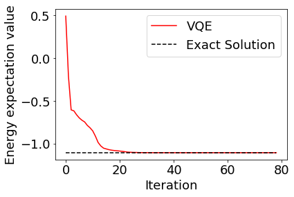
Plotting the execution result, we can see that it has converged to the correct solution.

plt.rcParams["font.size"] = 18
plt.plot(cost_history, color="red", label="VQE")
plt.plot(range(len(cost_history)), [molecule.fci_energy]*len(cost_history), linestyle="dashed", color="black", label="Exact Solution")
plt.xlabel("Iteration")
plt.ylabel("Energy expectation value")
plt.legend()
plt.show()

Encouraged readers should calculate the ground state by changing distance, the distance between the hydrogen atoms and find the interatomic distance at which the hydrogen molecule is most stable. (It should be about 0.74 Angstroms, depending on ansatz performance.)