7-3. Portfolio optimization using HHL algorithm

Some of the circuits here are constructed with a controlled_on setting. This is the multi-controlled gate experimental feature that has not yet been released as of quri_parts 0.17.0.

In this section, let us calculate the optimal portfolio (asset allocation) based on the data of past stock price fluctuations, referring to the paper [1]. Portfolio optimization is one of the problems that is expected to be solved faster than before by using the HHL algorithm learned in section 7-1. Specifically, this time, we consider the problem of what kind of asset allocation will give the highest return with the lowest risk when investing in stocks of the four GAFA (Google, Apple, Facebook, and Amazon) companies.

Stock Price Data Acquisition

First, we obtain the stock price data of each company.

• Use daily data of GAFA 4 companies

• To obtain stock price data, use pandas_datareader to obtain from Yahoo! Finance database.

• Adjusted closing price in dollars (Adj. Close) is used for the stock price.

import numpy as np
import pandas as pd
from pandas_datareader import data as pdr
import yfinance as yf
from datetime import datetime
import matplotlib.pyplot as plt

yf.pdr_override()
y_symbols = ['GOOG', 'AAPL', 'META', 'AMZN']

startdate = datetime(2022,1,1)
enddate = datetime(2022,12,31)
data = pdr.get_data_yahoo(y_symbols, start=startdate, end=enddate)

df = data['Adj Close'][y_symbols]
df.tail()

[*********************100%%**********************]  4 of 4 completed

	GOOG	AAPL	META	AMZN
Date
2022-12-23	89.809998	131.127060	118.040001	85.250000
2022-12-27	87.930000	129.307236	116.879997	83.040001
2022-12-28	86.459999	125.339409	115.620003	81.820000
2022-12-29	88.949997	128.889572	120.260002	84.180000
2022-12-30	88.730003	129.207779	120.339996	84.000000

fig, axes = plt.subplots(nrows=1, ncols=2, figsize=(15, 6))
df.loc[:,['AAPL', 'META']].plot(ax=axes[0])
df.loc[:,['GOOG', 'AMZN']].plot(ax=axes[1])

<Axes: xlabel='Date'>

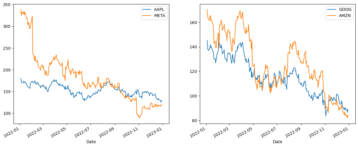
*The reason why the four stocks are divided into two groups here is because the stock price values are close to each other and easy to see when plotting, and there is no deeper meaning.

Data Preprocessing

Next, the acquired stock prices are converted to daily returns to obtain some statistics.

Conversion to Daily Returns

The daily return (rate of change) \(y_t\) (where \(t\) is the date) of an individual stock is defined as follows

\[y_t = \frac{P_t - P_{t-1}}{P_{t-1}}\]

This is obtained with the pct_change() method of the pandas DataFrame.

daily_return = df.pct_change()
display(daily_return.tail())

	GOOG	AAPL	META	AMZN
Date
2022-12-23	0.017562	-0.002798	0.007855	0.017425
2022-12-27	-0.020933	-0.013878	-0.009827	-0.025924
2022-12-28	-0.016718	-0.030685	-0.010780	-0.014692
2022-12-29	0.028799	0.028324	0.040131	0.028844
2022-12-30	-0.002473	0.002469	0.000665	-0.002138

df.values

array([[145.07449341, 179.95387268, 338.54000854, 170.40449524],
       [144.41650391, 177.66999817, 336.52999878, 167.52200317],
       [137.65350342, 172.94400024, 324.17001343, 164.35699463],
       ...,
       [ 86.45999908, 125.33940887, 115.62000275,  81.81999969],
       [ 88.94999695, 128.88957214, 120.26000214,  84.18000031],
       [ 88.73000336, 129.20777893, 120.33999634,  84.        ]])

Expected Returns

Find the expected return \(\vec R\) for each stock. Here we use the arithmetic mean of the historical returns:

\[\vec R = \frac{1}{T} \sum_{t= 1}^{T} \vec y_t\]

expected_return = daily_return.dropna(how='all').mean() * 252 # Multiply by 252 annual operating days for annualization
print(expected_return)

GOOG   -0.419937
AAPL   -0.270522
META   -0.822084
AMZN   -0.586943
dtype: float64

Variance/Covariance Matrix

The sample unbiased variance/covariance matrix \(\Sigma\) of the returns is defined by

\[\Sigma = \frac{1}{T-1} \sum_{t=1}^{T} ( \vec y_t -\vec R ) (\vec y_t -\vec R )^T\]

cov = daily_return.dropna(how='all').cov() * 252 # For annualized basis
display(cov)

	GOOG	AAPL	META	AMZN
GOOG	0.150897	0.109549	0.170553	0.140956
AAPL	0.109549	0.127250	0.136161	0.124414
META	0.170553	0.136161	0.414463	0.195457
AMZN	0.140956	0.124414	0.195457	0.251178

Portfolio Optimization

Now that we are ready, let’s tackle portfolio optimization.

First, the portfolio (i.e., asset allocation) is represented by a 4-component vector \(\vec{w} = (w_0,w_1,w_2,w_3)^T\). For example, if \(\vec{w}=(1,0,0,0)\), it means a portfolio with 100% of its assets invested in Google stock.

Let us consider a portfolio that satisfies the following equation.

\[\min_{\vec{w}} \frac{1}{2} \vec{w}^T \Sigma \vec{w} \:\:\: \text{s.t.} \:\: \vec R^T \vec w = \mu , \: \vec 1^T \vec w =1\]

This formula means

• “minimizing the variance of the portfolio’s return”

under the following condition

• “The expected return (average of returns) of the portfolio is \(\mu\)”

• “the sum of the weights invested in the portfolio is 1” (\(\vec 1 = (1,1,1,1)^T\))

In other words, the best portfolio is the one that minimizes the variance (risk) of the desired future return of only \(\mu\) as much as possible. Such a problem setup is called Markowitz’s mean-variance approach and is one of the foundational ideas of modern financial engineering.

Using Lagrange’s undetermined multiplier method, \(\vec{w}\) satisfying the above conditions can be obtained by solving the linear equation

\[\begin{split}\begin{gather} W \left( \begin{array}{c} \eta \\ \theta \\ \vec w \end{array} \right) = \left( \begin{array}{c} \mu \\ 1 \\ \vec 0 \end{array} \right), \tag{1}\\ W = \left( \begin{array}{ccc} 0 & 0 & \vec R^T \\ 0 & 0 & \vec 1^T \\ \vec{R} &\vec 1 & \Sigma \end{array} \right) \end{gather}\end{split}\]

where \(\eta, \theta\) are the parameters of Lagrange’s undetermined multiplier method. Therefore, to find the optimal portfolio \(\vec w\), we can solve the simultaneous equation (1) for \(\vec w\). We have now attributed the portfolio optimization problem to a linear equation for which the HHL algorithm can be used.

Creating the matrix W

R = expected_return.values
Pi = np.ones(4)
S = cov.values

row1 = np.append(np.zeros(2), R).reshape(1,-1)
row2 = np.append(np.zeros(2), Pi).reshape(1,-1)
row3 = np.concatenate([R.reshape(-1,1), Pi.reshape(-1,1), S], axis=1)
W = np.concatenate([row1, row2, row3])

np.set_printoptions(linewidth=200)
print(W)

[[ 0.          0.         -0.41993745 -0.27052205 -0.8220839  -0.58694271]
 [ 0.          0.          1.          1.          1.          1.        ]
 [-0.41993745  1.          0.15089651  0.10954939  0.17055346  0.14095575]
 [-0.27052205  1.          0.10954939  0.12724979  0.13616129  0.12441403]
 [-0.8220839   1.          0.17055346  0.13616129  0.41446314  0.19545675]
 [-0.58694271  1.          0.14095575  0.12441403  0.19545675  0.25117849]]

expected_return

GOOG   -0.419937
AAPL   -0.270522
META   -0.822084
AMZN   -0.586943
dtype: float64

## Check eigenvalue of W -> fits in [-pi, pi]
print(np.linalg.eigh(W)[0])

[-1.94743143 -0.30935002  0.03004076  0.09772754  0.42730033  2.64550076]

Creating the right-hand side vector

Given the expected return \(\mu\) of the portfolio below, we can calculate the least risky portfolio that will yield such a return. The \(\mu\) can be set freely. In general, the higher the expected return, the greater the risk, but we will use 10% as an example (this is a very bearish one, since it is a time when GAFA stocks are going gangbusters).

mu = 0.1 # Portfolio returns (parameters to be put in hand)
xi = 1.0
mu_xi_0 = np.append(np.array([mu, xi]), np.zeros_like(R)) ## Vector on the right side of equation (1)
print(mu_xi_0)

[0.1 1.  0.  0.  0.  0. ]

Extend the matrix so that it can be handled by a quantum system

Since \(W\) is 6-dimensional, it is computable in a quantum system with 3 qubits (\(2^3 = 8\)). Therefore, we also make a matrix and a vector with the extended two dimensions filled with zeros.

nbit = 3 ## Number of bits used for state
N = 2**nbit

W_enl = np.zeros((N, N)) ## enl stands for enlarged
W_enl[:W.shape[0], :W.shape[1]] = W.copy()
mu_xi_0_enl = np.zeros(N)
mu_xi_0_enl[:len(mu_xi_0)] = mu_xi_0.copy()

We are now ready to solve the simultaneous equation (1).

Calculating the minimum variance portfolio using the HHL algorithm

Now, let us solve the simultaneous linear equations (1) using the HHL algorithm. First, as a preliminary step, we prepare the following functions.

• A function input_state_gate that returns a quantum circuit that converts the quantum state to \(|0\cdots0\rangle \to \sum_i x_i |i \rangle\) according to the classical data \(\mathbf{x}\) This function should be built using the qRAM concept, but since we are using a simulator, we will implement it as a non-unitary gate this time. Also, standardization is ignored.)

• Function add_QFT_gate adds a gate to perform quantum Fourier transform.

• Function get_phase_estimate_circuit returns a phase estimation gate.

import numpy as np
from numpy.typing import NDArray
from quri_parts.circuit import QuantumCircuit


def add_QFT_gate(
    circuit: QuantumCircuit,
    start_bit: int,
    end_bit: int,
    inverse: bool = False
) -> None:
    """
    Making a gate which performs quantum Fourier transfromation between start_bit to end_bit.
    (Definition below is the case when start_bit = 0 and end_bit=n-1)
    We associate an integer  j = j_{n-1}...j_0 to quantum state |j_{n-1}...j_0>.
    We define QFT as
    |k> = |k_{n-1}...k_0> = 1/sqrt(2^n) sum_{j=0}^{2^n-1} exp(2pi*i*(k/2^n)*j) |j>.
    then, |k_m > = 1/sqrt(2)*(|0> + exp(i*2pi*0.j_{n-1-m}...j_0)|1> )
    When Inverse=True,  the gate represents Inverse QFT,
    |k> = |k_{n-1}...k_0> = 1/sqrt(2^n) sum_{j=0}^{2^n-1} exp(-2pi*i*(k/2^n)*j) |j>.

    Args:
      int start_bit:  first index of qubits where we apply QFT.
      int end_bit:    last  index of qubits where we apply QFT.
      bool Inverse: When True, the gate perform inverse-QFT ( = QFT^{\dagger}).
    Returns:
      qulacs.QuantumGate: QFT gate which acts on a region between start_bit and end_bit.
    """
    n = end_bit - start_bit + 1

    for target in range(end_bit, start_bit-1, -1):
        circuit.add_H_gate(target)
        for control in range(start_bit, target):
            angle=(-1)**inverse * 2*np.pi / 2**(target-control+1)
            circuit.add_U1_gate(target, angle, controlled_on={control: 1})

    for s in range(n//2):
        circuit.add_SWAP_gate(start_bit+s, end_bit-s)


def get_phase_estimate_circuit(
    n_total_qubits: int,
    unitary_matrix: NDArray[np.complex128],
    start_qubit: int,
    n_phase_estimate_qubit: int,
) -> QuantumCircuit:

    n_s = int(np.log2(unitary_matrix.shape[0]))
    n_p = n_phase_estimate_qubit

    circuit = QuantumCircuit(n_total_qubits)

    ## ------- Hadamard gate on register bit -------
    for register in range(start_qubit, start_qubit+n_p): ## from nbit to nbit+reg_nbit-1
        circuit.add_H_gate(register)

    ## ------- Implement phase estimation -------
    ## U := e^{i*A*t) and its eigenvalues are diag( {e^{i*2pi*phi_k}}_{k=0, ... N-1)).
    ## Implement \sum_j |j><j| exp(i*A*t*j) to register bits

    for register in range(start_qubit, start_qubit+n_p):
        ## Implement U^{2^{register-nbit}}.
        circuit.add_UnitaryMatrix_gate(
            np.arange(n_s),
            np.linalg.matrix_power(unitary_matrix, 2**(register - start_qubit)),
            controlled_on={register: 1}
        )

    add_QFT_gate(circuit, start_qubit, start_qubit+n_phase_estimate_qubit-1, inverse=True)

    return circuit

First, set the necessary parameters for the HHL algorithm. Set the clock register quantum bit number reg_nbit to 7 and the coefficient scale_fac used for scaling the matrix \(W\) to 1 (i.e., do not scale it). Also, the coefficient \(c\) used for the control rotation gate is kept at half of the smallest number of nonzeros that can be represented by the reg_nbit bits.

# number of registers used for phase estimation
reg_nbit = 7

## Factor to scale W_enl
scale_fac = 1.
W_enl_scaled = scale_fac * W_enl

## Minimum value to be assumed as an eigenvalue of W_enl_scaled
## In this case, since the projection succeeds 100%, we set the value as a constant multiple of the minimum value that can be represented by the register.
C = 0.5*(2 * np.pi * (1. / 2**(reg_nbit) ))

The core of the HHL algorithm will be written. In this article, we use the quri_parts.qulacs.simulator, so various simplifications have been made. This is an implementation to get a sense of how the HHL algorithm works.

• The part of preparing the input state \(|\mathbf{b}\rangle\) is simplified.

• The part of \(e^{iA}\) used in the quantum phase estimation algorithm is the diagonalization of \(A\) by a classical computer.

• Control rotation gate that takes inverses is also implemented by a classical computer..

• Measure the projection to the auxiliary bit \(|0 \rangle{}_{S}\) and treat only the states where the measurement result 0 is obtained. (For convenience of implementation, the definition of the action of the control rotation gate is reversed from section 7-1)

Construct the HHL circuit

Here, we create an HHL quantum circuit. Starting from the 0th bit, we have the bits in the space where A acts (0th ~ nbit-1th), the register bits (nbit th ~ nbit+reg_nbit-1 th), and the bits for conditional rotation (nbit+reg_nbit th).

from functools import reduce
from quri_parts.qulacs.simulator import run_circuit
from quri_parts.circuit import inverse_circuit

def get_condition_rotation_gate(n_qubits: int, n_bit: int, n_reg_bit: int) -> QuantumCircuit:
    """conditional rotation circuit

    The eigenvalue of A*t corresponding to the register |phi>
    is l = 2pi * 0. phi = 2pi * (phi / 2**reg_nbit).
    The definition of conditional rotation is (opposite of the text)
    |phi>|0> -> C/(lambda)|phi>|0> + sqrt(1 - C^2/(lambda)^2)|phi>|1>.
    Since this is a classical simulation, the gate is made explicitly.
    """
    condrot_mat = np.zeros( (2**(n_reg_bit+1), (2**(n_reg_bit+1))), dtype=complex)
    for index in range(2**reg_nbit):
        lam = 2 * np.pi * (float(index) / 2**(n_reg_bit) )
        index_0 = index ## integer which represents |index>|0>
        index_1 = index + 2**n_reg_bit ## integer which represents |index>|1>
        if lam >= C:
            ## Since we have scaled the eigenvalues in [-pi, pi] beforehand,
            ## [pi, 2pi] corresponds to a negative eigenvalue
            if lam >= np.pi:
                lam = lam - 2*np.pi
            condrot_mat[index_0, index_0] = C / lam
            condrot_mat[index_1, index_0] = + np.sqrt( 1 - C**2/lam**2 )
            condrot_mat[index_0, index_1] = - np.sqrt( 1 - C**2/lam**2 )
            condrot_mat[index_1, index_1] = C / lam

        else:
            condrot_mat[index_0, index_0] = 1.
            condrot_mat[index_1, index_1] = 1.
    circuit = QuantumCircuit(n_qubits)
    circuit.add_UnitaryMatrix_gate(range(n_bit, n_bit+n_reg_bit+1), condrot_mat)
    return circuit

def get_HHL_circuit(
    n_bit: int,
    n_reg_bit: int,
    hermitian_matrix: NDArray[np.complex128]
) -> QuantumCircuit:

    D, P = np.linalg.eigh(hermitian_matrix)
    U_mat = P @ np.diag(np.exp( 1.j * D )) @ P.T.conj()

    total_qubits = n_bit + n_reg_bit + 1
    circuit = QuantumCircuit(total_qubits)

    phase_estimation_circuit = get_phase_estimate_circuit(
        total_qubits,
        U_mat,
        start_qubit=n_bit,
        n_phase_estimate_qubit=n_reg_bit,
    )

    condition_rotation_circuit = get_condition_rotation_gate(
        total_qubits, n_bit, n_reg_bit
    )

    circuit.extend(phase_estimation_circuit)
    circuit.extend(condition_rotation_circuit)
    circuit.extend(inverse_circuit(phase_estimation_circuit))

    return circuit

hhl_circuit = get_HHL_circuit(nbit, reg_nbit, W_enl_scaled)

Run the HHL quantum circuit and retrieve the result

Here, we prepare the state for us to send into the HHL circuit. We use the simulator provided by quri_parts.qulacs.simulator.

## ------ Prepare vector b input to the 0th~(nbit-1)th bit ------
state = np.kron(
    [1 if i == 0 else 0 for i in range(2**(reg_nbit + 1))],
    mu_xi_0_enl
)
updated_state = run_circuit(hhl_circuit, state)

After the acting the circuit on the state, we need to project the state to the \(|0\rangle\) subspace of the auxiliary bit. The 0th to (nbit-1)th bit then corresponds to the calculation result |x>.

projector = reduce(
    np.kron,
    [
        np.array([[1, 0], [0, 0]]) if i < 1 else np.eye(2)
        for i in range(hhl_circuit.qubit_count)
    ]
)
final_state = projector @ updated_state

## The 0th to (nbit-1)th bit corresponds to the calculation result |x>.
result = final_state[:2**nbit].real
x_HHL = result/C * scale_fac

Compare results

Comparing the solution x_HHL by the HHL algorithm with the solution x_exact by diagonalization of the usual classical computation, we can see that they are roughly in agreement. (There are several parameters that determine the accuracy of the HHL algorithm (e.g. reg_nbit), so please try changing them and experiment with them).

## Exact solution
x_exact = np.linalg.lstsq(W_enl, mu_xi_0_enl, rcond=0)[0]

print("HHL:  ", x_HHL)
print("exact:", x_exact)
rel_error = np.linalg.norm(x_HHL- x_exact) / np.linalg.norm(x_exact)
print("rel_error", rel_error)

HHL:   [-0.2591962  -0.18557542  0.49450532  1.50115768 -0.54142008 -0.46074174  0.          0.        ]
exact: [-0.25188165 -0.1853244   0.37818531  1.58529401 -0.51953462 -0.4439447   0.          0.        ]
rel_error 0.08155603917693245

If we take out only the actual weighting part

w_opt_HHL = x_HHL[2:6]
w_opt_exact = x_exact[2:6]
w_opt = pd.DataFrame(np.vstack([w_opt_exact, w_opt_HHL]).T, index=df.columns, columns=['exact', 'HHL'])
w_opt

	exact	HHL
GOOG	0.378185	0.494505
AAPL	1.585294	1.501158
META	-0.519535	-0.541420
AMZN	-0.443945	-0.460742

w_opt.plot.bar()

<Axes: >

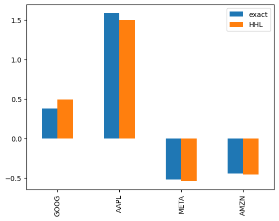
*Stocks with negative weights represent “short selling” (borrowing shares and selling them. It is a technique whereby profits can be made during periods of falling stock prices). In this case, the target return was set at 10%, which is quite small for GAFA stocks (expected return of 30-40% alone), so short selling is likely to have lowered the overall expected return.

Appendix: Back Testing

The verification of an investment rule derived from historical data using subsequent data is called “back-testing,” and is important for measuring the effectiveness of the investment rule. In this section, we will observe how much asset values change in the following year, 2018, when invested in a portfolio constructed from 2017 data as described above.

yf.pdr_override()
y_symbols = ['GOOG', 'AAPL', 'META', 'AMZN']

startdate = datetime(2023,1,1)
enddate = datetime(2023,12,31)
data = pdr.get_data_yahoo(y_symbols, start=startdate, end=enddate)

df2022 = data['Adj Close'][y_symbols]
df2022.tail()

[*********************100%%**********************]  4 of 4 completed

	GOOG	AAPL	META	AMZN
Date
2023-12-22	142.720001	193.600006	353.390015	153.419998
2023-12-26	142.820007	193.050003	354.829987	153.410004
2023-12-27	141.440002	193.149994	357.829987	153.339996
2023-12-28	141.279999	193.580002	358.320007	153.380005
2023-12-29	140.929993	192.529999	353.959991	151.940002

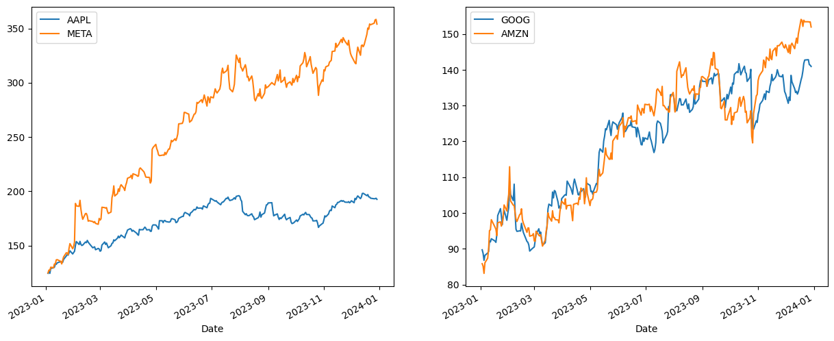
## Plot the stock price
fig, axes = plt.subplots(nrows=1, ncols=2, figsize=(15, 6))
df2022.loc[:,['AAPL', 'META']].plot(ax=axes[0])
df2022.loc[:,['GOOG', 'AMZN']].plot(ax=axes[1])

<Axes: xlabel='Date'>

# Changes in portfolio asset values
pf_value = df2022.dot(w_opt)
pf_value.head()

	exact	HHL
Date
2023-01-03	128.187768	123.985720
2023-01-04	128.782543	124.311268
2023-01-05	127.056521	122.515043
2023-01-06	131.919778	127.037984
2023-01-09	132.714873	127.853714

# Since the initial amount may differ between exact and HHL, we look at returns normalized by the value at the beginning of the period.
pf_value.exact = pf_value.exact / pf_value.exact[0]
pf_value.HHL = pf_value.HHL / pf_value.HHL[0]
print(pf_value.tail())

               exact       HHL
Date
2023-12-22  0.851713  0.799935
2023-12-26  0.839405  0.787424
2023-12-27  0.824654  0.770290
2023-12-28  0.827375  0.772570
2023-12-29  0.836015  0.782851

pf_value.plot(figsize=(9, 6))

<Axes: xlabel='Date'>

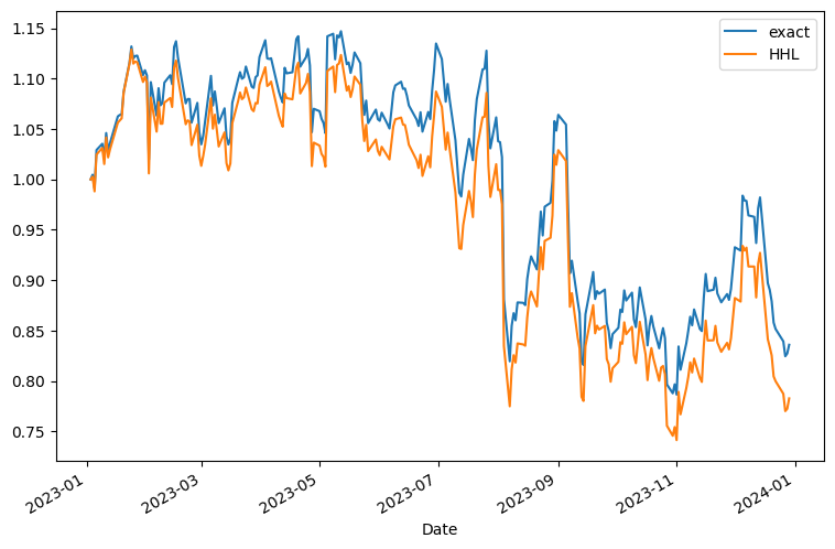
The stocks of all GAFA companies except Amazon were soft in 2018, resulting in a loss of roughly -20%. The EXACT solution seems to be somewhat better. Incidentally, since what we originally did was risk minimization, we also calculated the risk for the past year, and the EXACT solution resulted in smaller risk.

pf_value.pct_change().std() * np.sqrt(252) ## annualized

exact    0.409176
HHL      0.435979
dtype: float64

Reference

[1] P. Rebentrost and S. Lloyd, “Quantum computational finance: quantum algorithm for portfolio optimization“, https://arxiv.org/abs/1811.03975